Latent Space Approaches to Subtyping in Oncology Trials
Michael Kane and Brian Hobbs
Outline
Motivation: the "new" way clinical oncology trials are being conducted
The patient heterogeneity problem
Automated subtyping using latent space methods
Case study: predicting patient response by subtype
Case study: diagnosing mis-dosing based on adverse events
The "old" way of conducting clinical trials
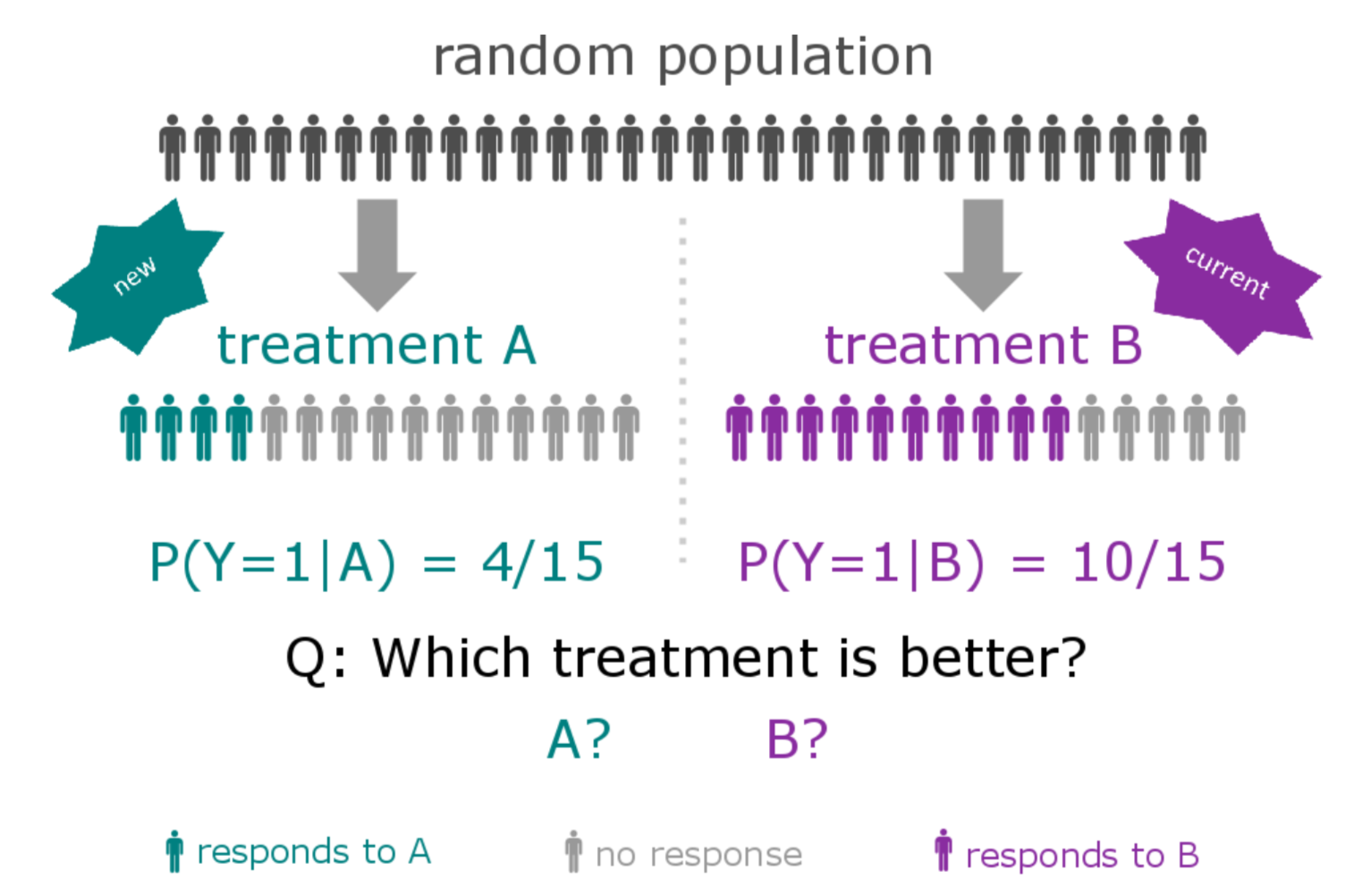
New compound is developed and is thought to deliver a (small) benefit over current therapies for a specific histology
A large number of patients are enrolled (at least hundreds)
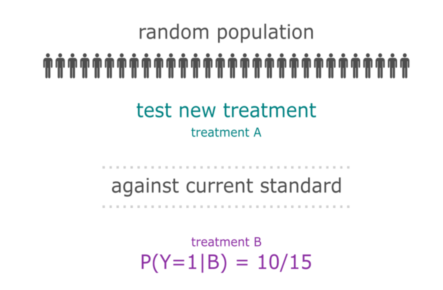
The response rate of the treatment population is tested against a control group
Entrectinib: Patient X Before
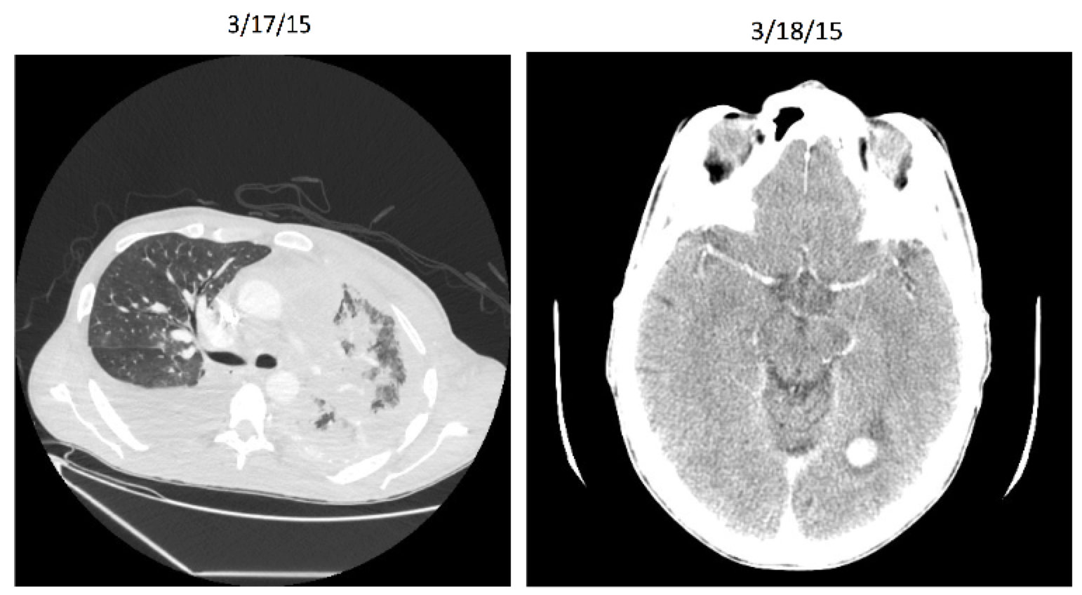
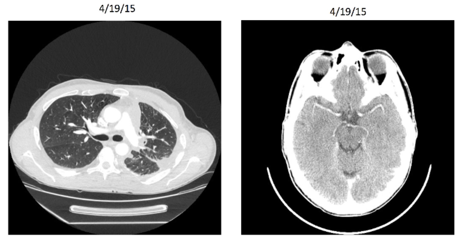
Entrectinib: Patient X After
Entrectinib
Targeted therapy (NTRK gene rearrangement)
Very stringent inclusion/exclusion criteria
Effective for other histologies (including breast, colorectal, and neuroblastoma)
8/11 responders for lung cancer in initial study
Breakthrough Trials
"A drug that is intended to treat a serious condition AND preliminary clinical evidence indicates that the drug may demonstrate substantial improvement on a clinically significant endpoint(s) over available therapies"
Benefits:
- Priority review: expedited approval process
- Rolling reviews, smaller clinical trials, and alternative trial designs
Alternative Designs
Often means single arm
Smaller populations
May include multiple histologies
Still work within FDA regulation, often including "all-comers"
| Biomarker | Tumor Type | Drug | N | ORR (%) | PFS (months) |
|---|---|---|---|---|---|
| BRAF V600 | NSCLC (>1 line) | Dabrafenib + Trametinib | 57 | 63 | 9.7 |
| ALK fusions | NSCLC (prior criz) | Brigatinib | 110 | 54 | 11.1 |
| ALK fusions | NSCLC (prior criz | Alectinib | 225 | 46-48 | 8.1-8.9 |
| EGFR T790M | NSLCLC (prior TKI) | Osimertinib | 127 | 61 | 9.6 |
| BRCA 1/2 | Ovarian (>2 prior) | Rucaparib | 106 | 54 | 12.8 |
| MSI-H/MMR-D | Solid Tumor | Pembroliumab | 149 | 40 | Not reached |
| BRAF V600 | Erdheim Chester | Vemurafinib | 22 | 63 | Not reached |
Breakthrough Therapies
The patient heterogeneity problem
The patient heterogeneity problem
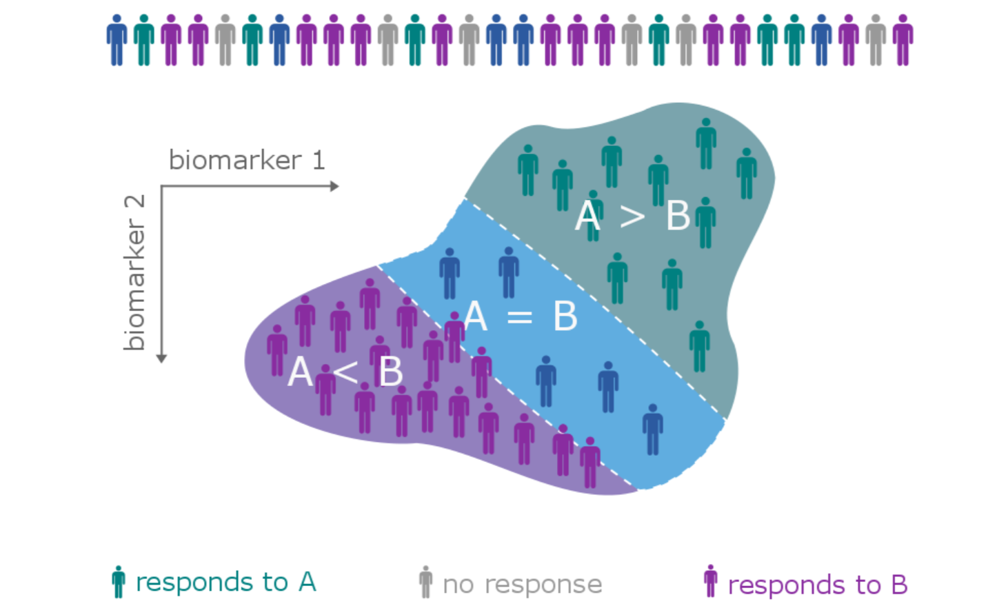
The patient heterogeneity problem
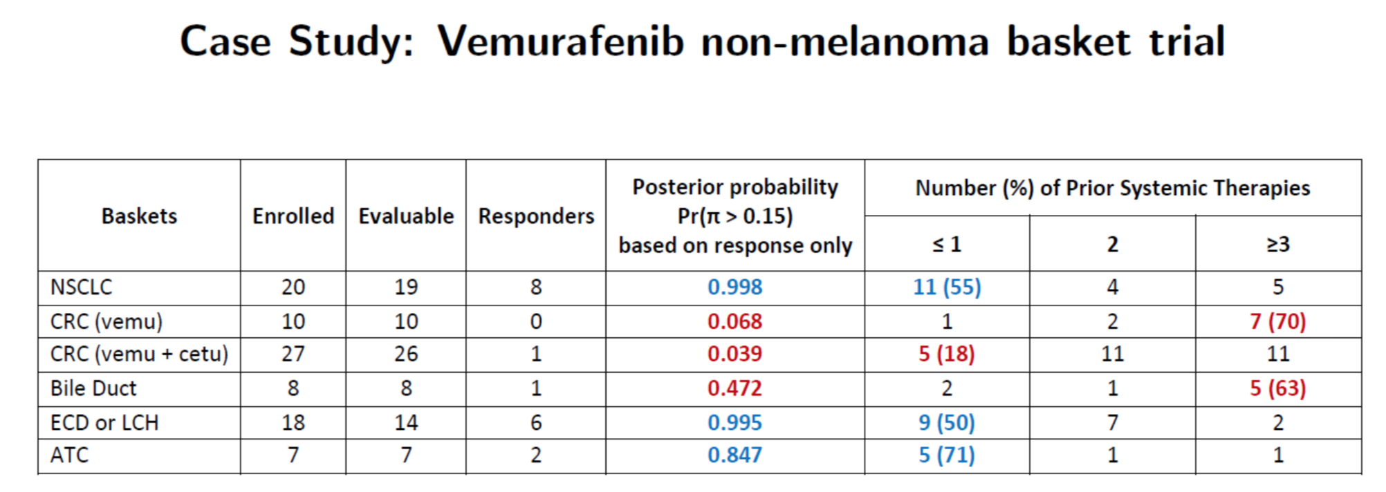
Hobbs, Kane, Hong, and Landin. Statistical challenges posed by basket trials: sensitivity analysis of the Vemurafinib study. Accepted to the Annals of Oncology.
A subtype is a group of patients with similar, measurable characteristics who respond similarly to a therapy.
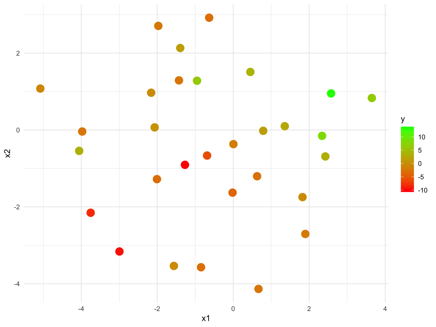
Why isn't supervised learning enough?
> summary(lm(y ~ x1n + x2n - 1, ts1))

Call:
lm(formula = y ~ x1n + x2n - 1, data = ts1)

Residuals:
   Min     1Q Median     3Q    Max
-7.276 -2.695  0.260  2.341  7.358

Coefficients:
    Estimate Std. Error t value Pr(>|t|)
x1n   1.1018     0.2266   4.863 4.03e-05 ***
x2n   1.2426     0.2398   5.181 1.69e-05 ***
---
Signif. codes:  0 ‘***’ 0.001 ‘**’ 0.01 ‘*’ 0.05 ‘.’ 0.1 ‘ ’ 1

Residual standard error: 3.647 on 28 degrees of freedom
Multiple R-squared:  0.6383,	Adjusted R-squared:  0.6124
F-statistic:  24.7 on 2 and 28 DF,  p-value: 6.572e-07
We can't tell this
from this
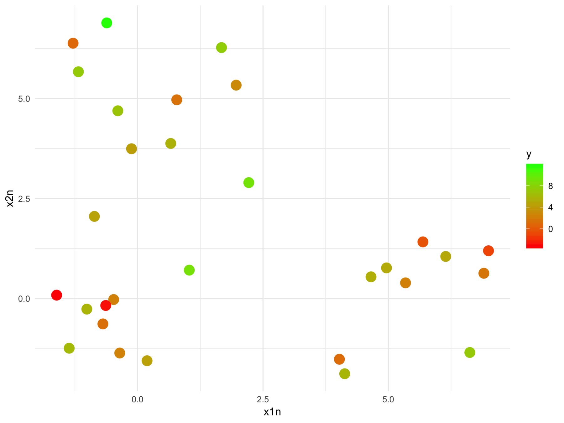
The model fits relationships between the regressors and the outcome
But we may want the relationships between the regressors with respect to the outcome
More formally start with supervised learning:
Consider \( n \) training samples \( \{x_1, x_2, .., x_n\} \), each with \(p\) features.
Given a response vector \(\{y_1, y_2, ..., y_n\}\), find a function \(h : \mathcal{X} \rightarrow \mathcal{Y}\) minimizing the \(\sum_{i=1}^{n} L( h(x_i), y)\) with respect to a loss function \(L\).
Construct \(h = f \circ g_y \) such that \(g_y : \mathcal{X} \rightarrow \mathcal{X'} \) is a latent space projection of the original data, whose geometry is dictated by the response.
Note that \(f\) is not parameterized by the response.
...and construct a (supervised) latent space
Let \(X \in \mathcal{R}^{n \times p}\) be a full-rank design matrix with \(n > p\), \(X = U \Sigma V\) is the singular value decomposition of \(X\).
where \(\Gamma\) is a diagonal matrix in \(\mathcal{R}^{p \times p}\), \(\mathbf{1}\) is a column of ones in \(\mathcal{R}^n\), and \(\varepsilon\) is composed of (sufficiently) i.i.d. samples from a random variable with mean zero and standard deviation \(\sigma\).
A simple example with OLS
Under the \(\ell^2\) loss function we can find the optimal value of \(\widehat \Gamma\) among the set of all weight matrices \(\tilde \Gamma\) with
The matrix \(\widehat \Gamma\) is \(\text{diag}(\widehat \beta)\) where \(\widehat \beta = \Sigma^{-1} U^T Y\) is the slope coefficient estimates of the corresponding linear model.
A simple example with OLS
\(X_Y = XV \tilde \Gamma\) represent the data in the latent space
Each column whose corresponding slope coefficient is not zero, contributes equally to the estimate of \(Y\) in expectation
A simple example with OLS
If the distance metric denoted by matrix \(A \in \mathcal{R}^{p \times p}\) and the distance between any two \(1 \times p\) matrices \(x\) and \(y\) expressed by
The square euclidean distance between two samples, \(i\) and \(j\) in \(X_Y\), denoted as \(X_Y(i)\) and \(X_Y(j)\) respectively is
A metric learning connection
A bias-corrected Gramian matrix estimate
Proof:
Let \(\mathbf{Z}\) be a diagonal matrix of standard normals
A toy example with iris
> head(iris)
  Sepal.Length Sepal.Width Petal.Length Petal.Width Species
1          5.1         3.5          1.4         0.2  setosa
2          4.9         3.0          1.4         0.2  setosa
3          4.7         3.2          1.3         0.2  setosa
4          4.6         3.1          1.5         0.2  setosa
5          5.0         3.6          1.4         0.2  setosa
6          5.4         3.9          1.7         0.4  setosa
>
> fit <- lm(Sepal.Length ~, iris[,-5])
A toy example with iris
> mm <- model.matrix(Sepal.Length ~ ., iris[,-5])
>
> km <- kmeans(mm, centers = 3)
> table(km$cluster, iris$Species)

    setosa versicolor virginica
  1     21          1         0
  2     29          2         0
  3      0         47        50
>
> # ...
> table(subgroups$membership, iris$Species)

    setosa versicolor virginica
  1     50          0         0
  2      0         23         0
  3      0         27        20
  4      0          0        30
Comparison with K-means
> mm <- model.matrix(Sepal.Length ~ ., iris[,-5])
>
> km <- kmeans(mm, centers = 4)
> table(km$cluster, iris$Species)

    setosa versicolor virginica
  1      0         24         0
  2     50          0         0
  3      0          0        36
  4      0         26        14
>
> # ...
> table(subgroups$membership, iris$Species)

    setosa versicolor virginica
  1     50          0         0
  2      0         23         0
  3      0         27        20
  4      0          0        30
Comparison with K-means
Back to cancer
Clinical trial data is not low-dimensional
Sometimes the predictive information isn't in a linear subspace of the data
Anonymous drug 1
Received "accelerated approval"
Subtype response based on baseline characteristics
All Trajectories
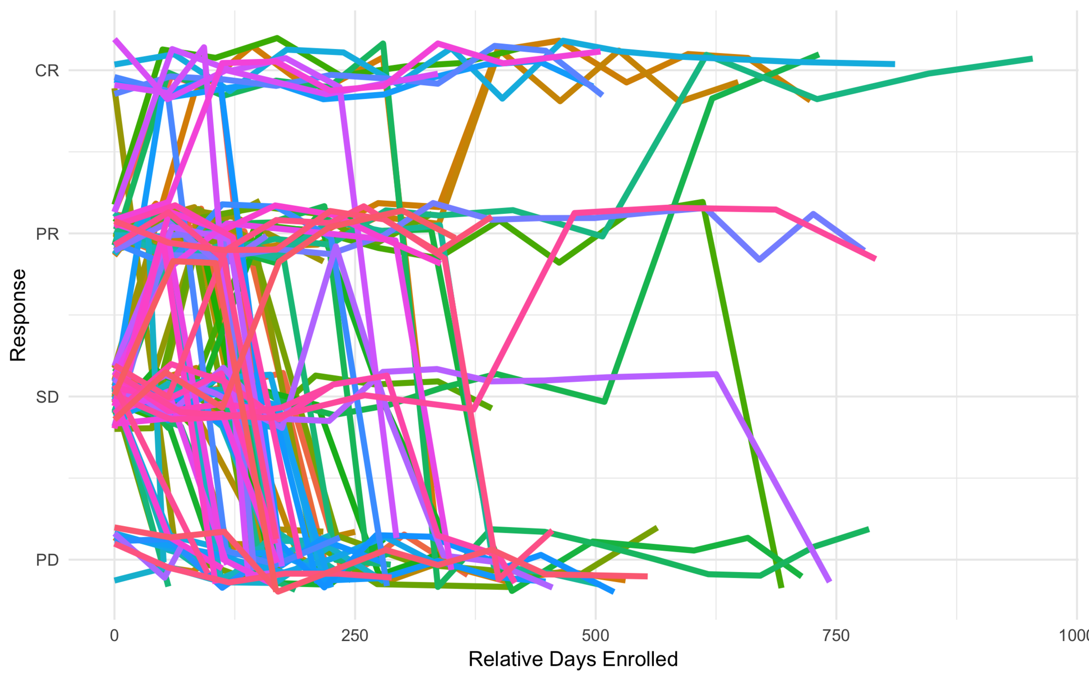
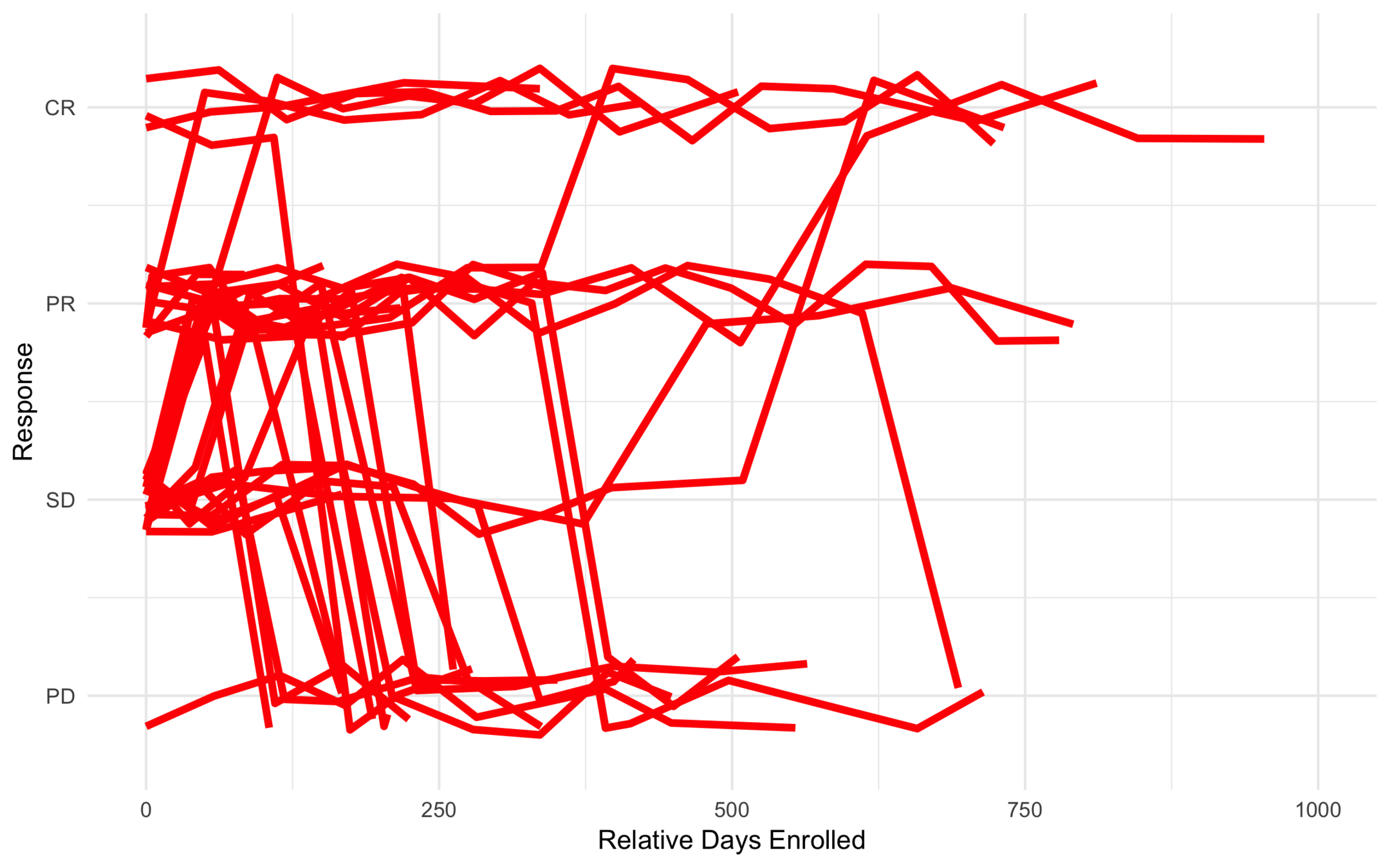
Low Risk
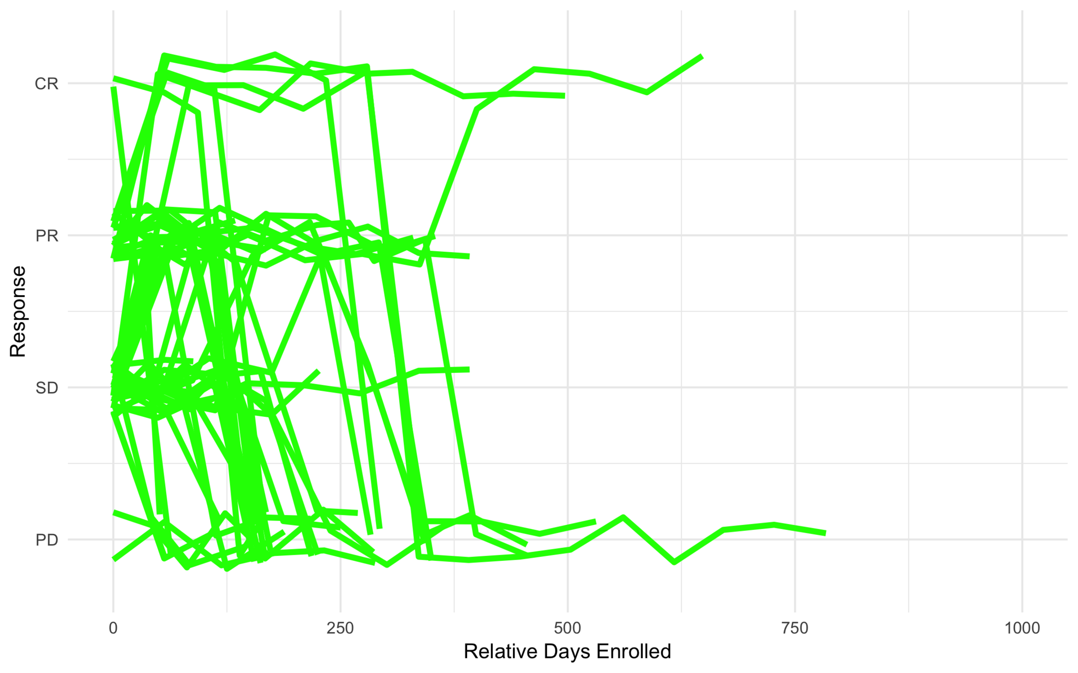
Intermediate Risk
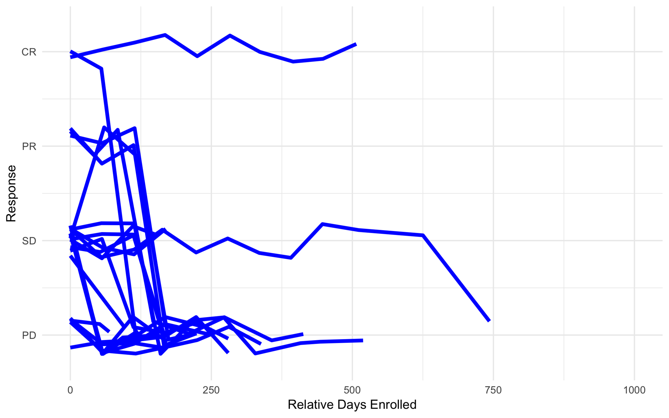
High Risk
Anonymous Drug 1
Was found to be effective for a certain type of cancer.
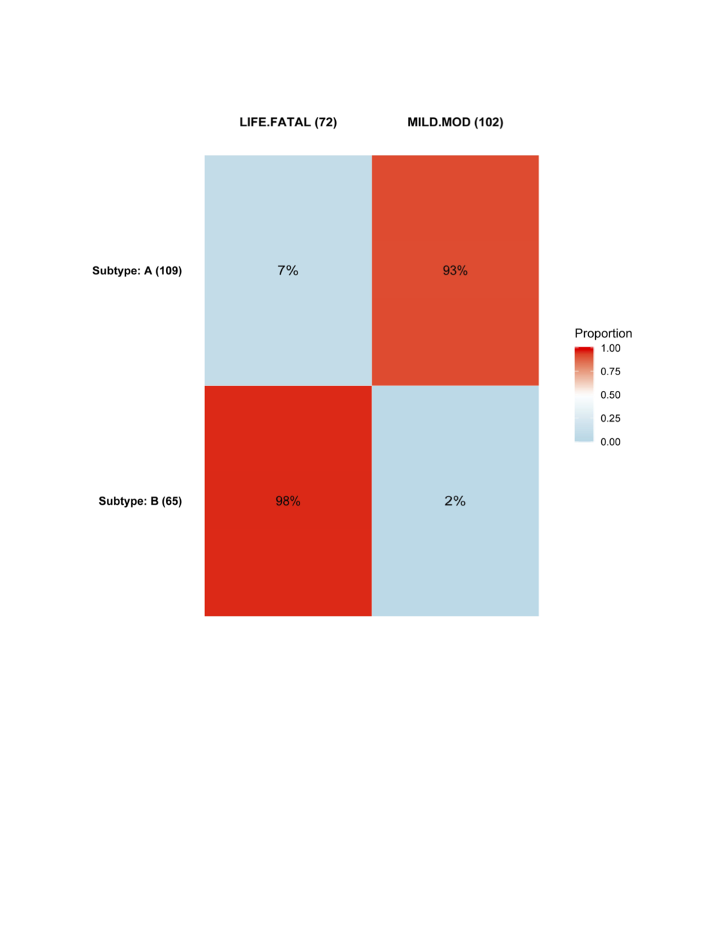
Ran into problems with severe toxicity events (449 toxicities out of 607).
Goal was to find subtypes least (or most) likely to have toxicity events.
| Variable | Description |
|---|---|
| AMD19FL | Exon 19 Del. Act. Mut. Flag |
| AM858FL | L858R Activating Mut. Flag |
| LIVERFL | Mets Disease Site Liver Flag |
| DISSTAG | Disease Stage at entry |
| NUMSITES | Num. of Mets Disease Sites |
| PRTK | Number of Prior TKI |
| PRTX | Number of Prior Therapies |
| WTBL | Baseline Weight |
| SEX |
AE Heatmap

AE Similarity Network

What else can you do with subtyping?
1. Improve prediction accuracy:
- Recall \(g_y : \mathcal{X} \rightarrow \mathcal{X'} \)
- Combine new samples with an \(f\) parameterized by \(Y\), \(h' = f_y \circ g_y \)
- E.g. Bayesian power prior
2. Construct counterfactuals and create synthetically controlled trials.
- Obtain data from other trials (standard of care)
- Project data into the latent space
- Match
- Compare results