Writing Regression Routines in R
Goals for the talk
This talk is is about writing linear regression routines in R and how they fit together
I'll cover intuition and implementations
- Ordinary least squares (OLS)
- Ridge Regression
- Generalized Linear Models
- Elastic Net
Implementations are meant to be short and readable
Anti-Goals
I'm not going to:
- spend a lot of time on statistical properties
- talk about optimality characteristics
- show code that's been optimized for speed
Why should we care about linear models?
They are old (Gauss 1795, Legendre 1805).
Random Forests (RF) are at least as simple and often do better at prediction.
Deep Learning (DL) dominates vision, speech, voice recognition, etc.
LM vs Rf
LM generally has lower computational complexity
LM is optimal RF is not
LM can outperform RF for certain learning tasks
RF is more sensitive to correlated noise
LM vs DL
See most arguments for LM vs RF
We understand characteristics of the space we are in with LM. Not so with DL.
RESULT: We know how things go wrong with LM, not with DL.
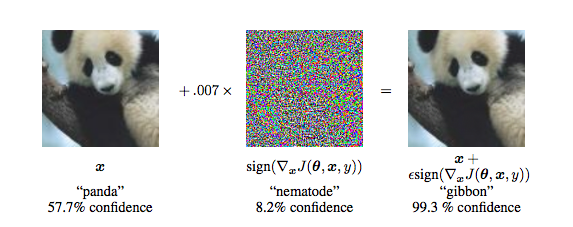
Breaking DL with Adversarial noise
Figure from Explaining and Harnessing Adversarial Examples by Goodfellow et al.

Advantages of LM
Computationally Efficient
LM is not simply a prediction tool - results are interpretable
Diagnostics for assessing fit and model assumptions
LM is compatible with other models
> train_inds = sample(1:150, 130)
> iris_train = iris[train_inds,]
> iris_test = iris[setdiff(1:150, train_inds),]
> lm_fit = lm(Sepal.Length ~ Sepal.Width+Petal.Length,
+             data=iris_train)
> sd(predict(lm_fit, iris_test) - iris_test$Sepal.Length)
[1] 0.3879703
> library(randomForest)
> iris_train$residual = lm_fit$residuals
> iris_train$fitted_values = lm_fit$fitted.values
> rf_fit = randomForest(
+   residual ~ Sepal.Width+Petal.Length+fitted_values,
+   data=iris_train)
>
> lm_pred = predict(lm_fit, iris_test)
> iris_test$fitted_values = lm_pred
> sd(predict(rf_fit, iris_test)+lm_pred -
+   iris_test$Sepal.Length)
[1] 0.3458326
> rf_fit2 = randomForest(
+   Sepal.Length ~ Sepal.Width+Petal.Length,
+   data=iris_train)
> sd(predict(rf_fit2, iris_test) - iris_test$Sepal.Length)
[1] 0.40927
The not so ordinary least squares model
Assume
Find
Derivation
What if X isn't full rank?
my_lm = function(X, y) {
  XTy = crossprod(X, y)
  XTX = crossprod(X)
  QR_XTX = qr(XTX)
  keep_vars = QR_XTX$pivot[1:QR_XTX$rank]
  solve(XTX[keep_vars, keep_vars]) %*%
    XTy[keep_vars]

}
What if X is "almost" not full rank?
Numerical Stability
> x1 = 1:100
> x2 = x1 * 1.01 + rnorm(100, 0, sd=7e-6)
> X = cbind(x1, x2)
> y = x1 + x2
>
> qr.solve(t(X) %*% X) %*% t(X) %*% y
Error in qr.solve(t(X) %*% X) : singular matrix 'a' in solve
>
> beta = qr.solve(t(X) %*% X, tol=0) %*% t(X) %*% y
> beta
        [,1]
x1 0.9869174
x2 1.0170043
> sd(y - X %*% beta)
[1] 0.1187066
>
> sd(lm(y ~ x1 + x2 -1)$residuals)
[1] 9.546656e-15
Should I include x1 and x2 if they are colinear?
> X = matrix(x1, ncol=1)
> beta = solve(t(X) %*% X, tol=0) %*% t(X) %*% y
> beta
     [,1]
[1,] 2.01
> sd(y - X %*% beta)
[1] 6.896263e-06
Dropping Unbiasedness
We can sometimes get better prediction if we allow some bias (Cramér-Rao bound).
Add a parameter α to control bias.
Can be solved with
my_ridge = function(X, y, lambda) {
  XTy = crossprod(X, y)
  XTX = crossprod(X)
  QR_XTX = qr(XTX)
  keep_vars = QR_XTX$pivot[1:QR_XTX$rank]
  solve(XTX[keep_vars, keep_vars] +
    lambda*diag(length(keep_vars)) %*%
    XTy[keep_vars]
}
Adding model selection
We can select which regressors do a good job predicting the dependent variable by adding another constraint
The Ridge Part
The Least Absolute Shrinkage and Selection Operator (LASSO) Part
my_lmnet = function(X, y, lambda, alpha, maxit=10000, tol=1e-7) {
  beta = beta_old = rep(0, ncol(X))
  quad_loss = Inf
  for(j in 1:maxit) {
    quad_loss_old = quad_loss
    beta = coordinate_descent(X, y, lambda, alpha, beta_old)
    quad_loss = quadratic_loss(X, y, lambda, alpha, beta)
    if(quad_loss > quad_loss_old) break
    beta = beta_old
  }
  list(beta=beta_old, iterations=j)
}
coordinate_descent = function(X, y, lambda, alpha, beta_old,
                              W=rep(1,nrow(X)) {
  beta = beta_old
  for (l in 1:length(beta)) {
    beta[l] = soft_thresh(sum(W*X[,l]*(y - X[,-l] %*% beta_old[-l])),
                          sum(W)*lambda*alpha)
  }
  beta / (colSums(W*X^2) + lambda*(1-alpha))
}

soft_thresh = function(x, g) {
  x = as.vector(x)
  x[abs(x) < g] = 0
  x[x > 0] = x[x > 0] - g
  x[x < 0] = x[x < 0] + g
  x
}

quadratic_loss = function(X, y, lambda, alpha, beta, W=1) {
  -1/2/nrow(X) * sum(W*(z - X %*% beta)^2) +
    lambda * (1-alpha) * sum(beta^2)/2 + alpha * sum(abs(beta))
}
how do we get from lmnet to glmnet?
A little bit about the glm
- g is the link function
- Element of W are inversly proportional to variance of response which depend on slope coefficients
- See Bryan's notes for more explanation
my_glm = function(X, y, family=binomial, maxit=25, tol=1e-08) {
  beta = rep(0,ncol(A))
  for(j in 1:maxit) {
    eta      = X %*% beta
    g        = family()$linkinv(eta)
    gprime   = family()$mu.eta(eta)
    z        = eta + (y - g) / gprime
    W        = as.vector(gprime^2 / family()$variance(g))
    beta_old = beta
    beta     = solve(crossprod(X,W*X), crossprod(X,W*z),
                     tol=2*.Machine$double.eps)
    if(sqrt(crossprod(beta-beta_old)) < tol) break
  }
  list(beta=beta, iterations=j)
}
IRLS
Now back to glmnet
my_glmnet = function(X, y, family=binomial, maxit=25, tol=1e-08) {
  beta = rep(0,ncol(X))
  for(j in 1:maxit) {
    eta      = X %*% beta
    g        = family()$linkinv(eta)
    gprime   = family()$mu.eta(eta)
    z        = eta + (y - g) / gprime
    W        = as.vector(gprime^2 / family()$variance(g))
    beta_outer_old = beta
    quad_loss = Inf
    for(k in 1:maxit) {
      beta_inner_old = beta
      quad_loss_old = quad_loss
      beta = coordinate_descent(X, z, lambda, alpha, beta_old, W)
      quad_loss = quadratic_loss(X, z, lambda, alpha, beta, W)
      if(quad_loss > quad_loss_old) break
      beta = beta_inner_old
    }
    if(sqrt(crossprod(beta_inner_old-beta_outer_old)) < tol) break
  }
  list(beta=beta_inner_old)
}
Wrapping up
Currently working on an out-of-core version ioregression.
I'll talk about making this fast at RFinance.
Thanks to Bryan Lewis for the GLM notes.
Thanks to AT&T Labs Research (Taylor Arnold and Simon Urbanek) for helping to make this happen.