Scalable, Exact Approaches to Fitting Linear Models when n >> p
Michael Kane, Taylor Arnold, and Simon Urbanek
iotools provides
-
A framework for computing on streamed chunks of data
-
Optimized routines for moving data from disk to processor
Let's build a regression library on top of it!
The design of ioregression
-
Build regression preprocessors, kernels, and combiners for different types of linear regressions.
-
Use iotools to stream data to the kernels and aggregate the results to get regression coefficients and diagnostics.
Why not just use foreach?
ioregression is foreach compatible
foreach doesn't give you
-
optimized io routines
-
Doesn't currently handle Hadoop's data locality
Goal is to provide numerical operations required for chunk-wise regressions.
Why linear regressions?
Linear Regressions are Simple
-
Assumptions are known
-
Diagnostics for assessing fit and assumptions
-
Results are interpretable
Linear Regressions are Computationally Efficient
-
Complexity is O(np^2)
-
Model fitting can be parallelized
Linear Regressions are Compatible with Other Analyses
> train_inds = sample(1:150, 130)
> iris_train = iris[train_inds,]
> iris_test = iris[setdiff(1:150, train_inds),]
> lm_fit = lm(Sepal.Length ~ Sepal.Width+Petal.Length,
+             data=iris_train)
> sd(predict(lm_fit, iris_test) - iris_test$Sepal.Length)
[1] 0.3879703
> library(randomForest)
> iris_train$residual = lm_fit$residuals
> iris_train$fitted_values = lm_fit$fitted.values
> rf_fit = randomForest(
+   residual ~ Sepal.Width+Petal.Length+fitted_values,
+   data=iris_train)
>
> lm_pred = predict(lm_fit, iris_test)
> iris_test$fitted_values = lm_pred
> sd(predict(rf_fit, iris_test)+lm_pred - iris_test$Sepal.Length)
[1] 0.3458326
> rf_fit2 = randomForest(
+   Sepal.Length ~ Sepal.Width+Petal.Length,
+   data=iris_train)
> sd(predict(rf_fit2, iris_test) - iris_test$Sepal.Length)
[1] 0.40927
Calculating the OLS slope coefficients
> x1 = 1:100
> x2 = x1 * 1.01 + rnorm(100, 0, sd=7e-6)
> X = cbind(x1, x2)
> y = x1 + x2
>
> qr.solve(t(X) %*% X) %*% t(X) %*% y
Error in qr.solve(t(X) %*% X) : singular matrix 'a' in solve
>
> beta = qr.solve(t(X) %*% X, tol=0) %*% t(X) %*% y
> beta
        [,1]
x1 0.9869174
x2 1.0170043
> sd(y - X %*% beta)
[1] 0.1187066
>
> sd(lm(y ~ x1 + x2 -1)$residuals)
[1] 9.546656e-15
What if we think of x1 and x2 as being highly correlated instead?
> X = matrix(x1, ncol=1)
> beta = qr.solve(t(X) %*% X, tol=0) %*% t(X) %*% y
> beta
     [,1]
[1,] 2.01
> sd(y - X %*% beta)
[1] 6.896263e-06
What does this buy us?
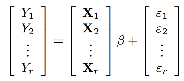
The regression calculation becomes
\hat{\beta} = \left(\sum_{i=1}^r X_i^T X_i \right)^{-1} \left(\sum_{i=1}^r X_i^T Y_i\right)
β^=(∑i=1rXiTXi)−1(∑i=1rXiTYi)
It is easy to implement OLS (and other regressions) in an embarrassingly parallel way.
How do I use it?
library(ioregression)
file_name = "2008.csv"
data = adf(file_name, sep=",", header=TRUE)
system.time({iofit = iolm(DepDelay ~ Distance, data=data)})
##    user  system elapsed
## 124.884   2.810 127.802
How fast is lm?
system.time({
df = read.table(file_name, header=TRUE, sep=",")
lmfit = lm(DepDelay ~ Distance, data=df)
})
##    user  system elapsed
## 134.436   3.577 138.258
Status
Under development
- Routines:
- OLS
- Ridge
- LARS
- GLM
- glmnet (coming)
- Platforms
- iotools (done)
- others?
Scalable, Exact Approaches to Fitting Linear Models when n >> p
By Michael Kane


